Every now and then I see some simple quizzes pop-up on Facebook such as: “Name a state without letter A in it.” The letter can be another, they just switch it around from time to time.
This particular post is inspired by such posts. Sure we can go through all the states in our heads and remember them manually, but that’s sort of a waste of time and frankly isn’t very exciting. The more fun thing to do is to figure out how to build a flexible, scalable solution to these types of questions…crafted in Excel.
Of course I could write the solution in C/C++, C#, Python, or in another language. Or if you’re into DB, you could use SQL variants and do a query. But if you don’t know programming or don’t want something that heavy weight for this silly quiz, you can still automate it like a wizard! In this post, I show a few simple methods (there are many other ways to slice it, and you can also try to come up with alternative solutions.). As a bonus, I’ll even create and run a SQL query from inside Excel to answer a little more complex question.
Social quizzes aside, by the end of this post, you’ll see how useful these Excel solutions are in the real-world for any analyst or manager for a multitude of scenarios.
Let’s start with the quizzes.
| QUIZ 1: | Name all states with the following letter in their names. (i.e. Letter can appears ANYWHERE in the name) |
| Y |
The first step to solving it in Excel is to have a table of all the state names. We can use SEARCH(letter, range). Where ‘letter’ would be the cell reference where the letter to match would be (e.g. if we’re searching for ‘Y’, and it is in cell B9, you would use B9 as the first argument. And ‘range’ is the range of cells covering the state names (e.g. C12:C61). SEARCH() returns the index position (1-based) of the letter in the name if found. If not found, it’ll return #VALUE as follows shown in Figure 1. The results are shown in column: SOLUTION 1a.
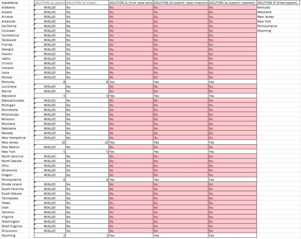
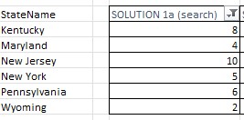
It’s now easy to pick out the names (Kentucky, Maryland, New Jersey, New York, Pennsylvania, Wyoming). To make it even easier, we can apply a filter on that column and weed out the “#VALUE” items and we’re left with a clean set of matching state names (states that have letter ‘Y’ in their names). Figure 2.
If the #VALUE bothers you, in addition to filtering them out, we can also completely eliminate it with a formula by wrapping our SEARCH function with IFERR() as in IFERROR(SEARCH(letter, range), “No”)…basically, IFERROR() will catch #VALUE as an error and replace it with the given word “No”.
This puts the word “No” next to the row of each state where the match was not found, and puts the index position if found as shown column SOLUTION 1b in Figure 1.
We can clean this up further by putting more user-friendly “Yes” or “No” next to each state and apply conditional formatting using this formula: IF(ISNUMBER(FIND(LOWER(letter),LOWER(range))),”Yes”,”No”). This is shown in column SOLUTION 1c in Figure 1. Note that instead of SEARCH(), I used FIND(), just to point out that FIND() is case-sensitive, therefore to look for ‘Y’ or ‘y’, I need to ensure that both the letter being searched and the state names are converted to the same case…in this case lower-case using LOWER(). We could also use UPPER() and obviously, we’d have to do it for both the letter and state names.
But if you prefer, you can simplify it using SEARCH() instead of FIND() and not worry about LOWER() or UPPER() as showin in column SOLUTION 1d in Figure 1. The formula is: IF(ISNUMBER(SEARCH(letter, range)),”Yes”,”No”)
We can yield the same result by using this formula: IFERROR(IF(SEARCH(letter, range)>0, “Yes”, “No”), “No”). This works because SEARCH returns only two possible values: the index position where the letter was found, or if not found it returns #VALUE…which we then catch by IFERROR() and change it to “No”. So, SEARCH() will never return 0 which we catch by IF(SEARCH(…)>0) clause. In other words, if a match is found, a number greater than zero is returned then put a “Yes” on that row, otherwise put a “No”. Pretty easy but slick. This is shown in SOLUTION 1e column in Figure 1.
One of my favorite and most powerful functions is FILTER(). Using this we simply extract a subset (instead of marking row by row) from the dataset that’s needed. To extract only the names where letter ‘Y’ appears for example (and assume Y is entered in cell B9), we can do this: FILTER(range,ISNUMBER(SEARCH(B9, range))) and boom! We have a clean list of the state names with that matching criterion as shown in SOLUTION 1f column in Figure 1. Personally, that’s my preferred method but sometimes we need to mark specific rows in which cases, any of the previous solutions will work. Another limitation of FILTER() is that it can’t handle wildcards, which we will need soon below as we get into more complex questions.
Now, you may be wondering: what if I want to get state names where a specific letter does NOT appear? When you think about it, all of the previous solutions 1a to 1e will work as-is. All you have to do is flip the “Yes” to “No”. and “No” to “Yes”.
However, FILTER() will take some tweaking to extract only the non-matching names. So, let’s make this the next quiz:
| QUIZ 2: | Name all states WITHOUT a specified letter in their names. (Letter appears ANYWHERE) |
| A |
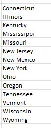
Now, we want the state names where letter ‘A’ does NOT appear using FILTER(). We can do this by strategically negative the result! NOT() changes TRUE to FALSE, and FALSE to TRUE. This is exactly what we need! So, this formula will do the magic: FILTER(range, NOT(ISNUMBER(SEARCH(letter, range)))) and the output is shown in Figure 3.
Let’s continue with more twisters!
| QUIZ 3: | Name a state starting with the following letters: |
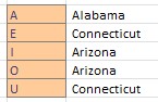
| A, E, I, O, U |
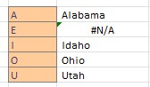
To solve this, I’ll use a completely different strategy…using VLOOKUP() with a wildcard! We want to check for each of the letters noted above (the vowels) and append the wildcard “*” after each and do a lookup. So, our search string will be: “A*”, “E*”, and so on since we want to match only those state names that start with that letter (as opposed to appearing anywhere in the state name). Assuming that the letter ‘A’ is in cell B94, the formula is: VLOOKUP(B94&”*”, range, 1,0). The output is shown in Figure 4. The ‘&’ is concatenating the wildcard to the value in cell B94. The 3rd argument is specifying column number 1, and 4th argument is doing an exact match (which is same as enter FALSE as that argument). We can clearly see there is no state name starting with letter E as it’s returning #NA. The formula would be copied for each row as shown for the given letter to match.
Similar to QUIZ 3, how about we look for the same letters but get the state names where those letter appear anywhere in a state name?
| QUIZ 4: | Name a state with the following letters ANYWHERE in its name: |
| A, E, I, O, U |
We can use the same idea, except now the query string will be “*[letter]*” and the formula is VLOOKUP(“*“&B94&”*”, range, 1,0). The output is shown in Figure 5 below.
Tired of quizzes yet? I didn’t think so! There are more questions to ask. How about the following?
| QUIZ 5: | Name a state whose name ends with one of the following letters |
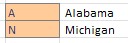
| A, N |
By now you probably have figured that this is another wildcard query. Correct, in this case the query string would be “*[letter]” since we’re matching only the last letter. So, this formula does the trick for each letter (row by row): VLOOKUP(“*”&B94, range, 1,0) assuming the letter is in B94. For the next letter, it can be B95, and so on and you’d copy or drag down the formula as needed to change the first parameter. The output is shown in Figure 6. One that ends in A, and one that ends with N. Note that VLOOKUP does not extract like FILTER can, it just returns the first match…which is exactly what we’re looking for here anyway.
We have done all kinds queries to answer many possible quizzes just using one table and one sheet in Excel! That’s powerful stuff. But I’m not done yet, how about patterns?
| QUIZ 6: | Get all states whose name contains the following pattern |
| SS |
Doing this in a typical Excel formula, while doable, is pretty clunky with too many nested formulas for my liking. For queries like this, query language like SQL is natural. Fortunately, if you know a bit of SQL, you can write and run SQL query from within Excel…without having to launch SQL Studio or the likes.
So, how do we do that? It takes a bit of navigating to find the right entry point and there are several ways to get to it. I’ll share an easy way.
Create a sheet or workbook with the state names. I happened to scrape the state names and their 2-letter symbols, so I have 2 columns: state abbreviations and their full names in their respective columns. For simplicity (for later steps), I turned the data range into a table with headers: StateAbb, StateName. I saved this file as “states.xlsx”.
Next, start Excel with a new/blank WB. From Data->Get Data->From Other Sources->From Microsoft Query (MQ). And choose “Excel Files*”. Ensure [x] Use the Query Wizard is checked on the pop-up dlialog. OK. Then choose the file (states.xlsx) via the pop-up file browser.
Choose the node with the name of the sheet that contains the table as discussed in step 1. (e.g. it will appear as “states$”) and add it to the Columns for query.
Click Next, Next until the last step where you have the option to either:
– Return Data to Microsoft Excel
– View data or edit query in Microsoft Query
Choose the 2nd one to edit it in Microsoft Query. Click Finish.
After Finish, the imported table will show up in Microsoft Query window. Figure 7.
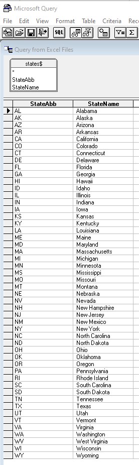
Click SQL button from menu bar to open the current SQL statement. It’ll look like:
SELECT `states$`.StateAbb, `states$`.StateName
FROM `[filename.xlsx]`.`states$` `states$`
Now, edit the text in the SQL pop-up editor as follows:
SELECT `states$`.StateAbb, `states$`.StateName
FROM `[path\filename]`.`states$` `states$`
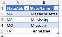
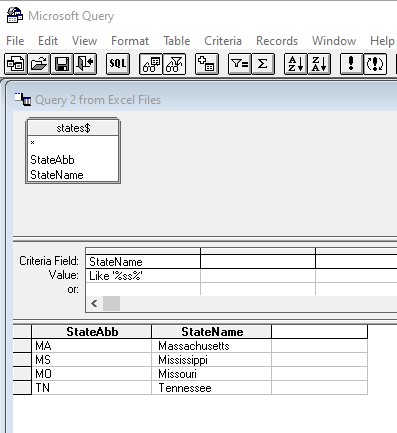
WHERE (`states$`.StateName Like ‘%ss%’)
Which says: Give me the names of states where there are two consecutive “ss” letters in their names, appearing anywhere in the names.
Click OK to see the results (if you edit, be sure to rerun it using “!” button). The query results are shown in Figure 8.
We can now simply copy the output table to share or save the output as an Excel file for reporting. To save the query to run it in the future, click on Save icon in the menu bar and save as it as a .dqy file somewhere. Then we can run it anytime by double-clicking, and get the results opened in a new Excel WB such as the one shown in Figure 8.
Once the query file is saved, we can always go back and rerun or edit the query. We can change the pattern to anything we want! Or create an entirely new query (New Query icon in MQ). The interface is shwon in Figure 9.
Some tips of dqy (saved queries): If your source datafile is moved to a different location, running the query will fail epicly with a jarring message as this:

See my complementary post on how to fix this here. I decided to keep that post separate from this to prevent this from getting even longer! But be sure to get that tip.
Have you been following this so far? If so, congratulations! You are a master of queries in Excel 🙂 Hope it was educational and helpful. Be sure to ask more questions and find their answers yourself! It’s a fun way to learn.
▛Interested in creating programmable, cool electronic gadgets? Give my newest book on Arduino a try: Hello Arduino!