Machine Learning in Excel? Isn’t ML the new thing, new algorithm that’s only done in the Cloud using R and Python? Nope! We’ve been doing in Excel for many years!! It’s only recently getting a lot of attention with Cloud and large datasets and made much, much simpler to use for today’s Data Scientists— but we (just analysts and techies) have been doing it in Excel the harder way (but with deeper understanding of each step) all along and can still continue to if we like. Let’s look at a real scenario.
We have data on consumer loans and consumers’ basic info such as income, credit score, and status of the loans. What the loaner wants to know the risk of loaning to specific categories of consumers. Actuaries do this all the time, and while I’m not and never desire to be one, I find that the underlying method of assessing the risks and applying that process to a machine learning experience such that computers can reuse the algorithms infinitely very fascinating. In this post, I’ll walk you through the process without requiring any computer language or hard-core math/statistical skills.
This is what we have (for brevity, the sample is kept small)…
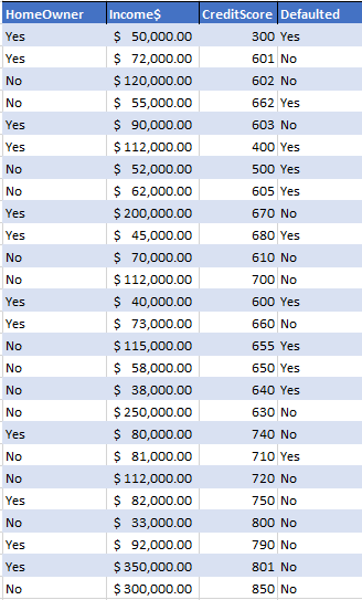
The general idea is to correctly predict how many loanees will default or not based on this data and can our process be applied as a machine algorithm to do this for billions->infinite number of records. Again and again and again…
The process starts with understanding of Entropy, which involves determining probabilities, and adding more and more information (parameters) to the logic and calculate and re-calculate the Entropy values…ultimately finding the lowest Entropy value where the
Information Gain is highest that includes all the relevant/available information (== parameters) in our dataset.
This is how machine algorithms, and machine learnings (ML) work. The goal for ML is to get to the right decision using the quickest route (== an efficient decision tree).
Let’s reflect back to the given data. The numbers are not really going to be that useful if we count the beans in income or even in credit scores. Instead we need to bucketize them.
Ultimately, the format we want for the dataset is a categorical bracketed dataset such as below:
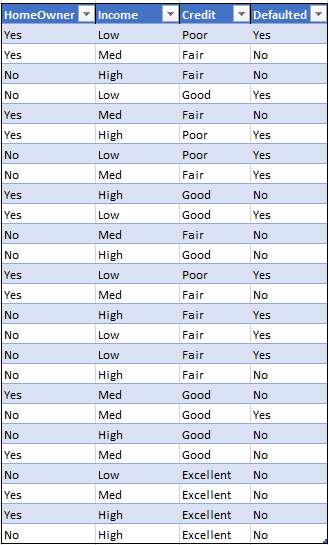
This is done by creating a range of values (From and To ranges) and each range given a value. This can be achieved in Excel for example by using vlookup(), IF(), IFS() or combination thereof. (I discuss and will share Excel intricacies in past and future posts separately….this one is focused on the process regardless of tools. This can be done in any other tool including in your favorite programming language).
Below is a step-by-step “manual” walkthrough of the core steps that may be going on behind the scenes on a computer applying Machine Learning algorithms. Except in this post, I’ll be doing the steps by hand and demonstrate them clearly. This is a good time to place where credit is due. I was inspired to do this experiment and write the blog by a talk by Paula Guilfoyle. Whose no-nonsense explanations are wonderful. She also has explanation of forming the decision tree based on similar scenarios here.
(Although I do have certifications on Artificial Intelligence, Data Science, and Machine Learning, but since I don’t get to practice it daily, it’s always great to see, learn from others’ talks and experiences in the domain who live it more frequently.)
As a first step, if we just look at it and create a probability of default just by looking at Defaulted status we can find the general overall likelihood of a loanee defaulting. In our dataset, we have 26 records, 11 of them have defaulted. Therefore the general probability of a loanee defaulting is about 42% (=11/26). And probability of not defaulting is 1-42% or 58%.
So, we can say 42% of loans will be defaulted based on our overall customer data. However, this is a crude estimate! We get more exact by going a little deeper. To do that, we can use Entropy and use it with added criteria of
our customers. As we add more parameters from the dataset, and recalculate Entropy for each and the Information Gain, we want to arrive at a much better predictor. This is how basically Machine Learning works.
We want to build a model that can quickly predict with good accuracy if a loanee will default or not. So, here I just introduced terms like: Entropy and Information Gain.
Entropy can mean a lot of different things depending on which discipline we want to tackle (linguistics, nature, thermodynamics, statistics, etc. etc.). You can read more about it in our trustee Wikipedia. However, the one I’m presenting here is more related to the explanation and purpose here (shout out to Benjamin Ricaud for that post).
So, yes our Entropy here is a measurement of random, scattered, noisy our data is! We can calculate it. Why? Because with starting Entropy value, we want to converge into a solution. A decision tree! A conclusion that’s based on less chaotic, noisy data. Therefore, our goal in this process is to calculate Entropy, add some parameters, re-calcuate, and add more, and repeat until we have a low Entropy value. The opposing view, loosely speaking, is the Information Gain. As we incrementally converge to a solution, Entropy is calculated and re-calculated. The difference between the current and previous Entropy is the Information Gain. Therefore, we want to INCREASE the Information Gain (while reducing the Entropy). While humans can make these decisions at many sophisticated situations extremely quickly, this is not possible for us to do with huge amount of data with complex shapes, and certainly no fun to repeat it a billion times! That’s why we invented the computers…that’s why we have Machine Learning (running on computers).
We can discuss this till we turn blue, but let’s get back to calculations. With the probabilities of defaulting (42%) and not-defaulting (58%) on loans found above, we can move on to calculate the Entropy value. The formula is:
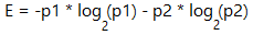
where p1 is probability of one outcome (42%), p2 is that of another (58%). And that’s Log base 2 (NOT 10). Then our E=0.982…(we’ll keep it limited to 3 decimals hereon). It tells us that our prediction that 42% will default in general may not be very accurate as the value is “noisy”. We know it’s noisy and has much randomness in it because E is ≈ 1. We can do better! We have other parameters like home ownership, credit rating, and income that are not included in this E calculation yet.
Let’s consider home ownership. We have 12 homeowners, 14 who are not. Out of 12 homeowners 4 defaulted. Out of non-homeowners 7 defaulted. For each type of homeowner (Yes/No) we need to calculate the probability of them defaulting. And calculate the E value for each.
TIP 1: These can be done in Excel without having to manually count and calculate. To get the count of total, we can use COUNTA(range of records). To get specific count of records, we can COUNTIF() and COUNTIFS() for multiple criteria. For example, to get the count of customers who are homeowners AND also defaulted on the loan we can use: =COUNTIFS([homeowner],”Yes”, [defaulted],”Yes”) assuming homeowner is the column range of HomeOwner data in the table above, and [defaulted] is the range of Defaulted values. TIP 2: It helps to convert the dataset into a table. To find the probability of Defaulting, it’ll be (count_of_homeowners_who_defaulted / total_count_of_homeowners).
The output from our sample dataset for HomeOwner parameter looks like this:

So, we can say about 33% of loans will be defaulted with customers who are homeowners. 50% of loanees who are not homeowners will default. (see Fig 1)
Next step before we find the OVERALL E value for home-ownership is to multiply each E values above (0.918 and 1) by the probability for each factor. That is, the probabilities of HomeOwner=Yes, and HomeOwner=No. (the formulas above in TIP 2 above). Then the overall E is 0.991 for HomeOwner parameter included.
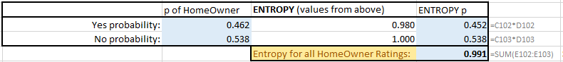
The formulas for each are also included in the right-most column above. C102 is the p of HomeOwner=Yes. D 102 is the E value calculated just step before this, so we arrive at 0.452 for that, and 0.538 for the HomeOwner=No. Summing them up, we get the overall E of 0.991.
Now that we have E from overall Defaulted and E from overall HomeOwnership, we can find the Information Gain value….which is simply the difference: IG=-0.008. Well, it’s negative!! That means, we haven’t got any new information by adding the HomeOwnership parameter (based on this sample data). Also, notice E is still very high ≈ 1. So, Home-ownership does NOT seem to be good parameter to use to determine loan risk!
But we need to continue! We haven’t included the credit rating and Income yet! Let’s apply the same methods to add credit rating parameters…
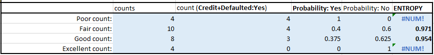
And then multiply each E with the probability of the parameter from occurring, then sum up the Es. And we get E=0.667
Note that the #NUM! errors in cell are normal to occur whenever a probability value is 0 due to the E formula. In such cases, before we move on to the next overall E calculation, we convert them to zeros.
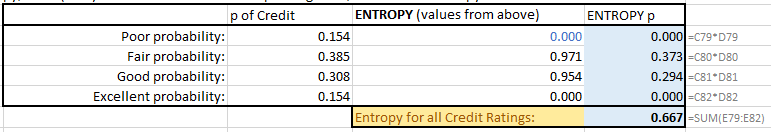
Now the Information Gain (IG) =0.316 (0.98 – 0.667) — this is positive! We’ve made good progress of narrowing down the scenarios.
Based on this, we can see: 40% of loans will be defaulted with customers with Fair credit score. And 100% with poor credit rating will default. (see Fig 3 Fair and Poor count rows and their Probability: Yes/No columns)
Next, what if we include Income as a parameter to this calculation?

As we can see now: 100% of loans will be defaulted with customers who have low incomes. (Fig 5)
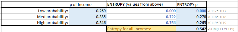
Now the Information Gain (IG) = 0.441. Meaning, we gained more information here by including income parameter. Since Entropy for Incomes is the lowest, that’s our best predictor so far. That is, Income and defaulting on loan are closely related. The next closest one is Credit rating. That’s also a good predictor. That is, Low credit rating and chance of defaulting are closely related.
Next, what if we look at Income and credit rating together? We already know 100% with low incomes and 100% with low credit rating will default.
What about customers of Med, High incomes with Fair, Good, Excellent credit ratings?
For that, we’ll add 2 more parameters, together. Going through the same iteration, but this time more COUNTIFS(), we arrive at the following matrices:
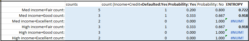
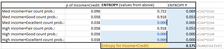
The Information Gain (IG) = 0.807 now! We gained the most information by including income AND credit rating.
CONCLUSION
The Entropy with Incomes + Credit rating information included is the lowest (0.175), that’s our VERY BEST predictor. The lowest risk we see for consumers with medium or higher income with fair or better credit rating is:
About 10% of loans will be defaulted with such demographics.
This is the lowest risk customers to loan to because:
About 90% of loans will be paid back. (i.e. These applications should be ACCEPTED.)
The highest risks are then: 100% loans will be defaulted if customer has either low income OR low credit rating. (i.e. These applications should be REJECTED).
In-between, we can say consumers who are homeowners should be CONSIDERED after credit criterion is met.
From this information, we can build an efficient decision tree.
I hope this was as interesting as I found it. I know there are some calculations details which may not be too clear here, but they can be done in Excel or any calculator/spreadsheet easily…the critical part is the concept. Happy learning!
▛Interested in creating programmable, cool electronic gadgets? Give my newest book on Arduino a try: Hello Arduino!
▟