There are times when I’d like to take a peek at my data CSV or XLS/X even before firing up Excel. Usually when the dataset is large and I want to quickly inspect it and modify it for my needs before even putting Excel to work. For that purpose, Python is very useful. Add its SQL capabilities to it, now we have a very powerful tool on hand even before launching Excel. After I’m done with data clean-up and filtering to my needs, I can apply further, detailed analysis and visualizations in Excel or PowerBI. In this blog, I walk you through the whole process using a dataset on UFO sightings that’s reported from 1930 through year 2000 in all the states of U.S. It contains 18K+ records and 9 columns.
The original data…(red dotted line denotes truncation)
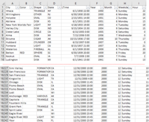
For this example, I don’t need to load all these columns…I would like to remove LTime, Year, Month, Weekday, and Hour fields…this will remove tons of overhead when loading the dataset! Additionally, I wanted to only look at the UFO sightings along the west coast from California all the way up to Alaska, but only more recent data starting from 1990. So, I only want a decade’s worth of data, localized to specific areas, working with only the fields relevant to my analysis.
This is where Python comes in really handy. Using its libraries for SQL and Excel (or CSV) files manipulation features, we can accomplish all that and more without launching any application other than just running the Python code.
What you’ll need
For smallest code footprint, we need to import: sqlite3, pandas, and create_engine from sqlalchemy libraries.
Explanation of code
After defining my source and destination data files, I create a SQL engine without actually creating any tangible database, or requiring any heavy SQL server. The engine resides only in memory, and I can feed SQL statements to it as in a database by creating a table in memory (called ufos) and manipulating, filtering, querying the data as desired. Using drop() method on the dataframe, I remove the columns I don’t care about from my table in memory.
Using Pandas, allows us to read in CSV or Excel files easily and load into dataframe objects in memory. Running that through the SQL hopper, also in memory, makes it very efficient.
As you’ll notice the source data simply includes data points of every instance that’s recorded. There’s no grouping by city, time, year, state or anything…they’re just distinct occurrences in order of recording. So, I need to find the number of sightings myself as well as the groupings as I like. Note also, that there are instances where not all fields have values (e.g. sometimes color and shape and even cities are noted and sometimes they are not). We can filter those out using SQL as shown above along with scoping the timeline from 1990 onward.
After SQL engine has done its thing, I take the result, convert it back to dataframe (because Pandas works with dataframes for Excel read/write) from a SQL object, and write to a new file as defined by output variable above.
During the course of code execution, we can verify the before-after effects in shell using dataframe’s shape attribute…e.g. df.shape and final_data.shape
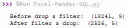
As you can see original data contained 18241 rows and 9 columns. I extracted 2526 rows (including header) and 5 columns that I care about, and created a new dataset off of that.
We can also get basic stats on data using dataframe’s describe() method. Depending on the data frame you want to look at, you can do df.describe() or final_data.describe() for the above code example to get an output like this:
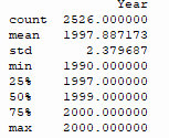
This shows the count of records for the column(s), its mean, standard deviation, min/max, and quartiles. For the Year column, for this dataset it might not be very relevant but it’s quite useful on datasets that contain lots of quantifiable data (e.g. measurements of any kind, populations, currency, etc.).
Ok, after the entire code is executed, we get a new Excel file as below…(red dotted line denotes truncation)
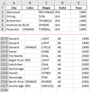
Great! Now I have a clean, tight, relevant dataset in a smaller Excel file that I can work with. Other variations of data I extracted from the original source were…
Group by States and find number of sightings, then sort by the number of sightings, accomplished by a SQL statement:
![]()
Show which year had the most/least sightings across USA, accomplished by a SQL statement:
![]()
Show how many sightings were recorded in WA state over the years, grouped by year and sorted by sightings, accomplished by a SQL statement:
![]()
Now that we have the data in Excel, we can create cool and useful vizualizations as below…

Observation: Most sightings across USA occurred in California followed by Washington state.
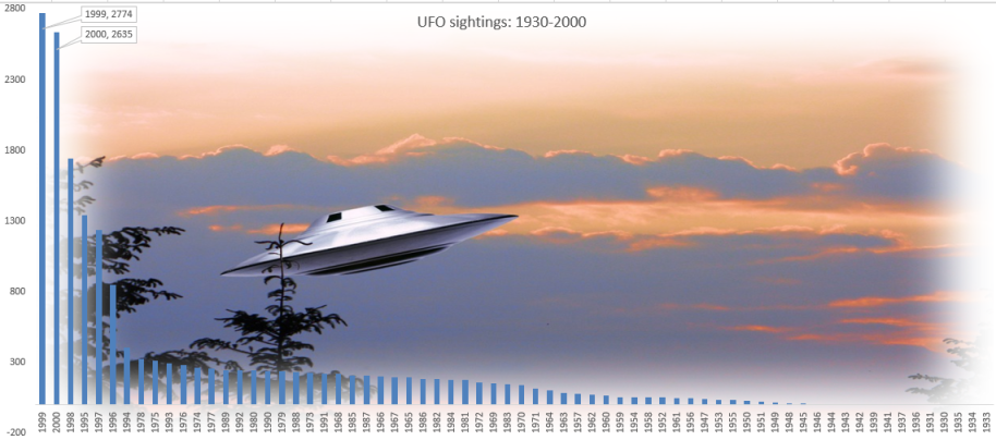
Observation: In USA, most UFO sightings since 1930 (to 2000) were reported in 1999 followed closely by year 2000.

Observation: In my state, Washington, most sightings were in 1995 followed closely by year 1999. The earliest officially recorded sighting appears in 1946 for WA.
Hope you found these tips useful. There are tons of other things we could do with Python and Excel; some are not really useful or necessary in my view as I find those accomplished in Excel directly much quicker and in more polished ways, but there are cases where Python’s features can add a big helping hand before Excel gets involved! In the future blogs, I’ll add some of those useful tips and scenarios in my blog.
This post is not meant to be a step-by-step, detailed tutorial, instead to serve key concepts, and approaches to problem-solving. Basic->Intermediate technical/coding knowledge is assumed.
If you like more info or source file to learn/use, or need more basic assistance, you may contact me at tanman1129 at hotmail dot com. To support this voluntary effort, you can donate via Paypal from the button in my Home page, or become a Patron via my Patreon site. A supporter/patron gets direct answers on any of my blogs including code/data/source files whenever possible upon request.