In this post, I share my method of creating charts in Excel to visualize multi-leg journeys with time-proportions and icons using data. Once the structure is in place, they are scalable and data can be updated without ever needing to manually create any designs or artwork.
Here’s the scenario
We want to plot a airplane journey from Seattle, Washington to Los Cabos, Mexico with a few stops in-between (Los Angeles, CA; Honolulu, HI; Mexico City, Mexico).
There is a layover between Honolulu and Mexico City, Mexico however with no immediate connection that has to be accounted for. The flight information is laid out in a table (each leg of the flight duration is converted to a common unit: hours) as this:
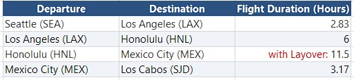
The chart should show a line connecting the origin and destination at each leg of the journey proportional to the flight times (in hours for example).
A basic version of the chart would look like this:
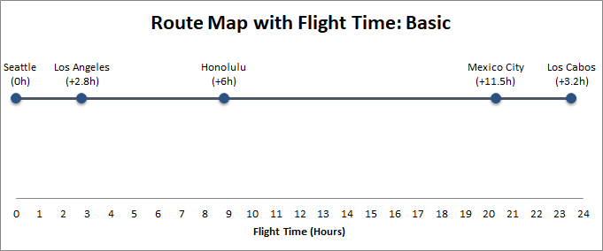
The flight times are accurately depicted along the x-axis. Each waypoint is depicted in the basic version with a circular node. The distance between waypoints is proportionally shown. This is achieved with a XY scatter plot.
If you can achieve this, the chart can be enhanced to look even more informative and attractive! I’ll share those below, but first let’s see how the basic chart can be done.
The Steps
Enter the data in a table with a layout as below:
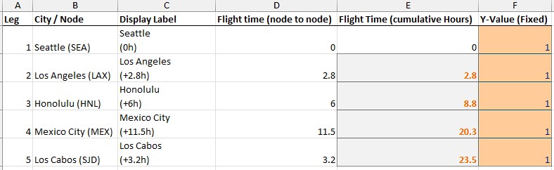
The Flight time (node to node), and Y-Value (Fixed) columns are the core data for the XY scatter plot.
The Flight Time (cumulative Hours) in column E is the duration of flight from the previous node to current node and accumulates node to node since beginning. So, it starts with 0 for starting point (Seattle), then for Los Angeles it’s 0+2.8, then for Honolulu it becomes 0+2.8+6=8.8 and so on. So, enter that as a formula in column E rows.
Due to a layover in this trip, the time between Honolulu and Mexico City is a larger number (11.5 hours).
Display Label column values are for Data Labels on the chart…these custom labels make the chart clean and readable.
Leg, and City/Node columns are just for our reference (not used in the chart directly).
All Y-values are set to a fixed value (1) to keep the timeline perfectly horizontal on the chart as a straight line on the chart. You can adjust the value as you wish making sure it makes visually sensible.
Select E, F columns (without the headers) and all their data rows and insert an XY scatter plot so that Series X values are column E values, and Series Y values are column F values.
Next, do a little cleanup on the chart
After the XY scatter plot is placed…
Adjust the max value for Y axis values (so the horizontal line between dots appear a little higher than the middle to indicate elevation); then remove the y-axis label.
Remove the major vertical and horizontal gridlines in the chart area — to make the chart look cleaner.
Click + next to chart to add [x] Data Labels, then More Options, click Label Options tab, expand Label Options node -> [x] Value From Cells and select the values from Display Label column.
Uncheck the Y Value and Show Leader Lines options there.
Double-click the x-axis label and edit Axis Options tab settings there to make the major units=1 (or whatever makes more sense for the route).
Keeping the x-axis values gives us the idea of total time end-to-end easily.
Finally, remove the Legends.
Now, the chart looks much cleaner and easy to read. However, we can improve this by making further tweaks to the whole process. We can add an airplane icon, for example overlaid on each leg of the journey!
Adding Airplanes to the chart
First we have to calculate the midpoint of the line that connects the origin and destination points.
Midpoint X = (X current node + X next node)/2
where X is the flight time values (hours) at each leg. So, to calculate Seattle to California (LAX), it’d be = (0 + 2.83)/2 = 1.42. The first leg is 0 because Seattle is the origin node.
Midpoint for CA to Hawaii (Honolulu) will be = (2.83 + 8.83)/2 = 5.83
The Airplane image/character will be placed exactly in the middle of the connecting link and on top of the line connecting the nodes in the XY Scatter plot, so the values are same as Y-Value (Fixed) as in the original XY Scatter plot.
Then Add the airplanes as a new series
Right-click anywhere inside the chart and choose Select Data.
Click Add to create a new series. Name it “Airplanes”.
Set the Series X values to the Airplane X-value rows (without the header).
Set the Series Y values to the Airplane Y-value column rows (all of them are same value). Click OK.
There will be a new line added on top of the existing lines connecting the nodes.
To remove it, click on it for each segment and double-click to bring up Format Data Point pane on right, then in Fill & Line tab, expand Line node and set it to: No line.
You’ll now see 4 new dots or square markers appearing directly on your timeline. Right-click one of these new midpoint dots and select Format Data Series.
Go to the Fill & Line tab > Marker > Marker Options > Change it to None. (This makes the dots invisible, leaving just the mathematical points).
Right-click any of those invisible midpoints from previous step (click exactly where the markers were on the line) and select Add Data Labels.
Right-click > Format Data Labels.
Under Label Options, check Value From Cells. Select the Label Character column values (no header) containing the airplane Unicode symbols (✈).
Uncheck the default Y Value and Show Leader Lines boxes.
Change the Label Position to Center.
Finally, set the font type and size to your liking, and format the airplane icon just like any text (it’s Unicode, not an image) by changing the font size and color to make them pop.
The chart now looks better. Here’s the enhanced version with airplanes…
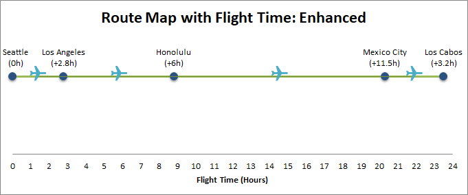
We can take it one step further! For example, we want to show the layover on the chart on the leg between Honolulu and Mexico City.
We can achieve that by showing a slightly different marker for the flight between Honolulu and Mexico City due to the layover delay by either showing these unicode chars instead of just one: ✈ character: ✈ ⏳ ✈. So enter those 3 unicode characters into the Label Character column’s cell for Honolulu, HI → Mexico City, Mexico row. I have kept the Label Character as-is for explanation, and created a new column Pro Label Character where I entered this, as I wanted to show the progression, but you can use the Label Character column and paste there without creating a new column. My final table looks like this…
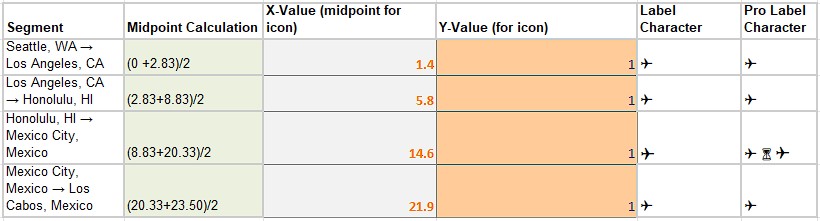
And the final Pro version of the chart should look like this:
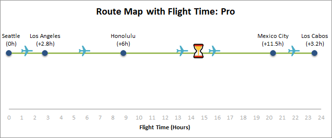
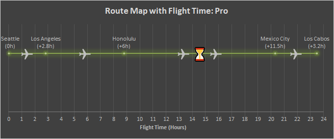
If you fancy, you can create a dark-mode chart; just select Chart Design and select a dark design and make the tweaks such as removing the Y-axis, adjusting the icon size, etc. to your liking. A dark-mode design looks like this:
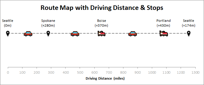
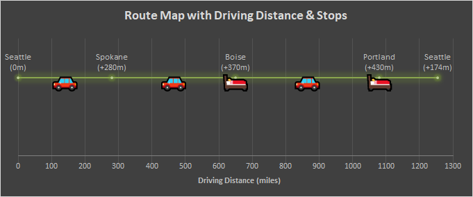
Now that you know how to create this type of chart. You can use the same method for road-trips or any mode of journey and even round-trips. For example, road trip charts with a hotel/overnight stay at Boise between for Seattle to Portland and back might look like these (light and dark modes)…
I hope this was educational. Happy charting! Until next time…
