In this post, I share an example of a very common challenge in business which is complex to solve just by hand, along with the easy solutions.
The Scenario: Let’s start with the scenario. We have a bakery that bakes 4 items that sell at our pre-determined prices as shown below:
| Cost (each) | |
| Bun | $3.00 |
| Cookie | $3.25 |
| Cheesecake | $3.75 |
| Biscottio | $2.50 |
The Challenge: We need to figure out the highest sales possible with these items given some realistic constraints. The constraints are:
- Price of any single item cannot exceed $7.50
- Quantity must be greater than 0 for any single item and cannot exceed 50.
- Cost of cheesecake cannot exceed $4.75.
- Total cost cannot exceed $175.
- Bun, Cookie, Biscotti price cannot exceed $6.
The Solution: In order to find the total maximum sales with the given constraints, we need to take several steps first. 1) Calculate total sales for each item. 2) Find the total sales for all items and then optimize it. 3) But to find the total sales, we need to also find the selling price for each to achieve the max sales. and 4) the quantity of each item that can be sold given the constraints. 5) Find the total costs of making all items as that is part of the constraint that must be an input.
In this example, we are mostly dealing with sales (not profit) but since we have the cost data of making each, we can also find the profit easily after solving the rest. The quickest way to solve this riddle is to use the Solver feature of Excel.
First, we have to shape the table appropriately to set up for Solver to work. The table reformatted should look as the Table 2 below:
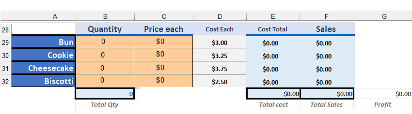
The B33 contains SUM() formula just to add all the quantities, cells in column E contain formulas to multiply corresponding B*D cells in each row, followed by the SUM() of column E29:32 rows in E33. Similarly, column F is B*C for each row followed the sum in F33. G33 is simply F33-E33.
As you see everything except what’s known (the Cost) is zero at this time. Because we’ll have the Solver fill in the data for B, C columns, and cell F33…which will be the maximum Total Sales value computed by the Solver. The rest will be filled in automatically by the formulas we entered above.
Now comes the first solution, we launch the Solver (Data->Solver) and carefully specify all its required parameters according to our scenario. We will choose Solving Method called GRG Nonlinear.
Also in the Solver dialog, set the following fields: Objective: F33 (Total Sales) and set it to find the Max. Then in ‘By Changing Variable Cells’ set the Quantity and price columns for all: $B$29:$C$32
In the ‘Subject to the Constraints’ field we enter the constraints such that each constraint is in its own line; so they are: C29:C32 <=7.50; B29:B32 >=1; B29:B32 <=50; D31<=4.75; E33<=175; C29<=6; C30<=6; C32<=6…then click OK to solve.
We are essentially letting Solver fill in the values for Quantity and Price each columns while being limited by the following constraints to find our value (Max of Total Sales).
If a solution is found (if the constraints are not achievable, then there will be no solutions), then there will be option to choose the reports for Excel to create which are: Answer Report, Sensitivity Report, Limits Reports. Also, if the problem is defined properly as explained above the Table 2 cells will be populated with the quantity, price, and our goal Total Sales values. The output is shown below in Table 3.
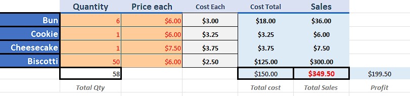
We find that maximum sales possible is $349.50 when we sell each item at specified prices at specified quantity. We would get a profit of $199.50 in that case. This is incredibly useful information not just about the feasibility of maximizing profit and/or sales but also at exactly what price point and at what volume of sales!
Bonus Challenge: We can run another scenario by finding the volume of each item we must sell to achieve lowest cost of production at the previously calculated maximum sales PLUS given the following constraints:
- We need to sell minimum 100 total items (quantity).
- We cannot produce more than 25 Cheesecakes (quantity).
- Quantity of any item cannot be zero.
In this case, we will let Solver adjust quantity with constraints but Price, Cost are fixed and the Total Sales must be >= $349.50 since that’s what Solver told us our maximum sales would be.
We set up the conditions as before, except this time we set the objective to Min and the cells to modify are in B column (Quantity). And we get the solution shown in Table 4 below.
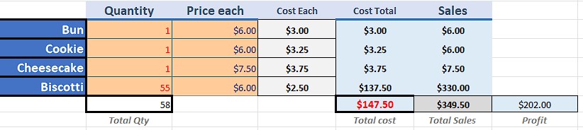
Solver has given us the the exact quantity of each item we should sell at the fixed price to achieve the target Total Sales of $349.50 while keeping the production cost at lowest.
With the solver, in addition to Max and Min value seeking, we can also set a specific value to seek which makes it very flexible and useful in many scenarios. In summary, Solver can change multiple parameters at a time to reach a specific target or answer. while Goal Seek can only tackle one parameter at a time. So, for multiple parameters and multiple constraints, use Solver.
So, when do we use Goal Seek then? Answer is for simpler scenarios. One parameter, no constraints. For example, if we wanted to find the number of Biscottis to sell to make $200 profit on it alone, we can use Goal Seek.
Suppose we have the following table. We want Goal Seek to fill in the Biscotti’s Quantity cell with the exact number that we need in order to have Profit on its row to be $200. See Table 5.
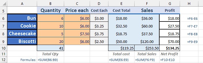
To find the answer, we open Goal Seek using Data tab. Then in the dialog, we enter the cell we’re trying to set up in ‘Set cell:’ field…in this case, G9 (profit from Biscotti sales). And in ‘To value:’ field we enter the number we chose: 200. Finally, in ‘By changing cell:’ field we enter the field that Goal Seek should fill in with the answer, which is the quantity of Biscottis we need to sell to make $200 profit off it. So, it’ll be the cell B9.
If a solution is found, Goal Seek will confirm and press OK to accept it and update the table. Now it should look as follows (Table 6):

As you can see, we need to sell 57 Biscottis to make $200 profit from it. The cells Goal Seek updated are shown in dark blue cells, bold font in Table 6.
Hope this was useful and gives you many ideas to use both the Solver and Goal Seek. I will also be writing a post about how to use What If in the near future.
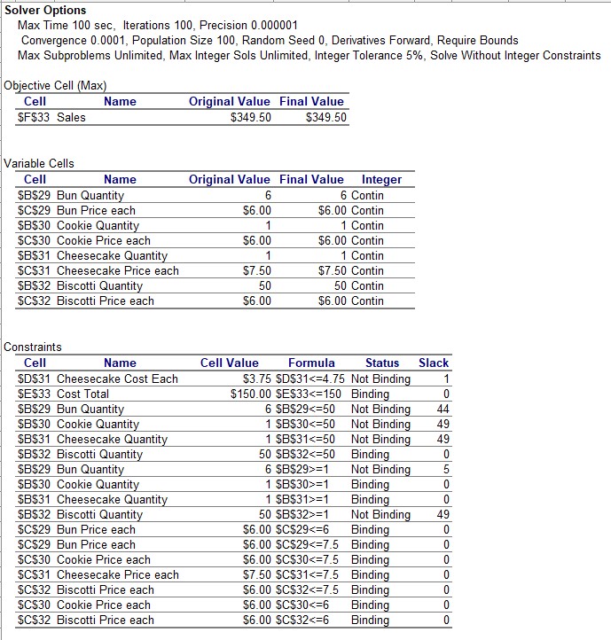
FYI, in Solver, if you chose to generate a Answer Report by the solver, a sample report (for the first Challenge above) would look like this: