Network graphs are quite fascinating to me. They are all around us and used daily in a multitude of real-world applications from supply-chain, routing, mapping, social media, scheduling, to networking. In this two-part blog series, I’ll go over some real-world applications of graphs and how to generate them dynamically using Python.
There are many complex mathematical algorithms that are in use for different scenarios; however, I won’t discuss the algorithms, rather, I’ll share ways to leverage them for practical purposes.
A few of the scenarios I cover in this blog series here:
Project scheduling example – Shows how to compute critical path on a network of related tasks. Covered here in Part 1.
Routing example – Shows how to create and draw a network graph with weighted edges. Computes shortest, longest paths, degrees, and more (using Dijkstra, DAG, BellmanFord, and Jin Yen’s algorithms). Covered here in Part 1.
Social network example – Creates and draws a sample social network. Covered in Part 2.
Family “tree” example – Shows how to create a relationship graph with color-codes and more. Covered in Part 2.
Each scenario is briefly explained below.
Project scheduling example:
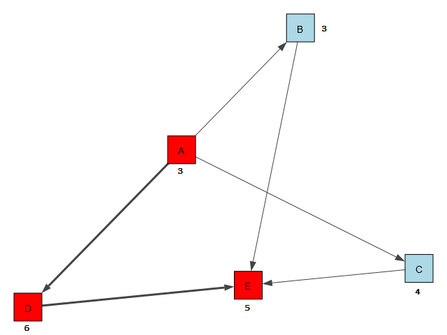
Often used in project management and scheduling, CPM is a common methodology to find the critical path of a “project” made of tasks or work-items from start to finish. In this example, we have a project consisting of tasks A, B, C, D, E. Each task has different amount of work and is expressed in amount of time required to complete the task. This value, duration, for the above tasks are, say, 3, 3, 4, 6, 5.
Objective: Find the critical path.
Solution: In Excel, and in Microsoft Project, there are built-in functionality to find this value. However, I wanted to solve all these problems in Python. I’ll be using “criticalpath” library (more info on it here). After installing the library the bit to get the critical path nodes and total duration is quite easy. First, we have to create the nodes with their durations values and connect them using its link() method. Sample code is below:
from criticalpath import Node
p = Node('project')
a = p.add(Node('A', duration=3))
b = p.add(Node('B', duration=3, lag=0))
c = p.add(Node('C', duration=4, lag=0))
d = p.add(Node('D', duration=6, lag=0))
e = p.add(Node('E', duration=5, lag=0))
p.link(a, b).link(a, c).link(a, d).link(b, e).link(c, e).link(d, e)
p.update_all()
l= p.get_critical_path() # get a list of nodes for critical path
print(l)
d=p.duration # get total duration
print(d)
The path is then printed in the shell as [A, D, E] and duration is 14. Pretty straight forward, however, this is not a visual graph…it just spits out the text output. What I want to do is actually visualize it. Specifically, I want to create a graph in memory, draw on screen, and also highlight the critical path edges and nodes.
To do that, I have to deal with real graph objects using igraph library (I’ll also show networkx library example later for another scenario). iGraph will me create the graphs, however, in order to actually draw it on screen, I need to pass the graph object over to a popular library called matplotlib.
First, the I create the edges of the nodes (or vertices), then the nodes with names, and create a custom node attribute called duration (each node will have its duration value associated), and a custom edge attribute called CP (each edge will have a flag to indicate if it’s in critical path or not…so that I can highlight the edge with thicker lines!). That part of the code is shown below:
import igraph as ig
g = ig.Graph([(0,1), (0,2), (0,3), (1,4), (2,4), (3,4)], directed=True)
g.vs["name"] = ["A", "B", "C", "D", "E"]
g.vs["duration"] = [3, 3, 4, 6, 5]
g.es["CP"] = [ False, False, True, False, False, True ]
Next, we need to draw it on screen and do the conditional formatting on the fly. That part is done with the code below:
import matplotlib.pyplot as plt
visual_style = {}
visual_style["vertex_size"] = 40
visual_style["vertex_label"] = g.vs["name"]
visual_style["edge_width"] = [1 + 2 * int(CP) for CP in g.es["CP"]]
visual_style["bbox"] = (640, 480)
visual_style["margin"] = 40
visual_style["vertex_shape"]="rectangle"
color_dict={"A":"Red", "B":"Lightblue", "C": "Lightblue", "D": "red", "E": "red"}
visual_style["vertex_color"] = [color_dict[name] for name in g.vs["name"]]

ig.plot(g, **visual_style)
And I’m done! The output is shown below:
Let’s move on to a little more sophisticated graph in the next scenario…
Routing example:
In this example, we’ll create a network of nodes with weighted edges. The weighted edges can be used as an indicator such as: task duration in days, task importance, network traffic, capacity, distance, etc. In this case, I’ll be using a networkx library to create the chart, and again draw using matplotlib.
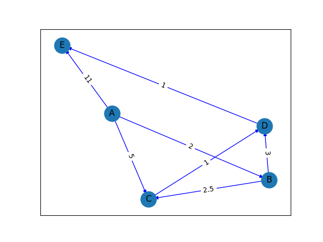
Imagine we have the following nodes: A, B, C, D, E and the nodes are inter-connected with edges and each edge has its unique weight value such that: A-B are connected and their edge value is 2. B-D are connected and their edge value is 3. A-C are connected and their edge value is 5. B-C are connected and their edge value is 2.5. D-E are connected and their edge value is 1. C-D are connected and their edge value is 1. Finally, A-E are connected and their edge value is 11.
Objectives: i) Find the shortest path from A to E. ii) Find the longest path from A to E. iii) Get all possible paths across the graph.
Solution: The following lines will create the graph in memory and finally plot it using plt.show() where plt is defined as: import matplotlib.pyplot as plt
import networkx as nx
G = nx.DiGraph()
G.add_weighted_edges_from([ ('A', 'B', 2), ('B', 'D', 3), ('A', 'C', 5), ('B', 'C', 2.5), ('D', 'E', 1), ('C', 'D', 1), ('A', 'E', 11) ])

pos = nx.spring_layout(G)
labels = nx.get_edge_attributes(G, 'weight')

nx.draw_networkx_nodes(G, pos, node_size=500)
nx.draw_networkx_edges(G, pos, edgelist=G.edges(), edge_color='green')
nx.draw_networkx_edge_labels(G, pos, edge_labels=labels)
nx.draw_networkx_labels(G, pos)
The graph output is shown below:
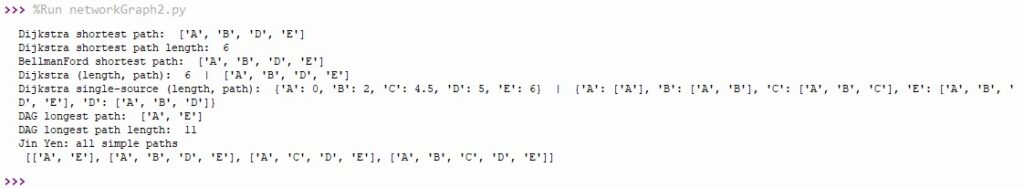
Once this is defined, we can retrieve important information about the nodes, edges, the entire graph programmatically. Some examples shown in code below…
print("Dijkstra shortest path (A to E): ", nx.dijkstra_path(G, 'A', 'E'))
print("Dijkstra shortest path length (A to E): ", nx.dijkstra_path_length(G, 'A', 'E'))
print("BellmanFord shortest path (A to E): ", nx.bellman_ford_path(G, 'A', 'E'))
length, path = nx.bidirectional_dijkstra(G, 'A', 'E')
length, path = nx.single_source_dijkstra(G, 'A')
print("Dijkstra single-source (length, path): ", length, " | ", path);
print("DAG longest path: ", nx.dag_longest_path(G))
print("DAG longest path: ", nx.dag_longest_path_length(G))
paths = list(nx.shortest_simple_paths(G, 'A', 'E'))
print("Jin Yen: all simple possible paths\n", paths)
And the information we get are below. We now know the longest path if 11 units and is A->E. The cheapest/shortest route is of 6 units: A->B->D->E and many more valuable information.
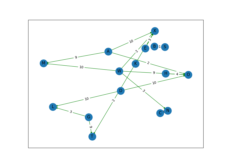
For further experimentation, I also created additional graphs along with randomization, an example of such is shown below with 20 random nodes of routers and/or computers.
I will be discussing the social network and family tree examples in the next blog. Be sure to read the Part 2 here.